Technology

A brief overview of the technical foundations behind our published results. Full details live in the technical reports themselves — this page just orients you and points to the source.

The dataset and the four AI models

All of our published block-level databases are built from the same source: 5,004 ground-truth images from the NIH ChestX-ray8 dataset, each partitioned into non-overlapping 8×8 pixel blocks — 81,975,528 blocks per model.

Citation: Wang, X., Peng, Y., Lu, L., Lu, Z., Bagheri, M., & Summers, R. M. (2017). ChestX-ray8: Hospital-scale chest x-ray database and benchmarks on weakly-supervised classification and localization of common thoracic diseases. Proceedings of CVPR, 3462–3471. Dataset available from the NIH Clinical Center.

Each image was reconstructed by four AI super-resolution models, run under two architectures:

Upscayl Standard (GAN-based)
Upscayl High-Fidelity (GAN-based variant)
Upscayl Digital-Art (GAN-based variant)
SwinIR (Transformer-based)

Upscayl is an open-source AI image upscaler; we chose it for being both popular and free to use. Standard, High-Fidelity, and Digital-Art are three of its bundled models, all GAN-based, used as they come with no further selection criteria — running the same analysis across several variants of a single tool was expected to surface whatever pattern held up on its own. SwinIR is a separate, widely used Transformer-based super-resolution model (Liang et al., 2021), included specifically to test whether our findings hold across a fundamentally different architecture — not just across variants of the same one.

Each model was also run under two conditions, referred to throughout the technical reports as noTTA and TTA (test-time augmentation): a common inference-time technique that reconstructs an image multiple times from augmented versions of the input and averages the results. In the super-resolution literature specifically, this technique is usually called self-ensemble, following EDSR's original "geometric self-ensemble" strategy — "TTA" is the more general term used across computer vision as a whole.

As elsewhere on this site: publishing per-model results is not a ranking or recommendation of any of these models. See FAQ.

Large-scale local analysis with DuckDB

Switching from SQLite

We started out analyzing this data with SQLite, but as the datasets grew into the hundreds of millions of blocks, individual queries began taking tens of minutes to hours — no longer a practical pace to work at. We switched to DuckDB, a column-oriented analytical database, and the same scale of data now runs in seconds to minutes on an ordinary PC. That's what let us screen-record an actual SQL query and show the result live, in the technical reports themselves — a more direct form of transparency than just publishing code or data, closer to demonstrating the experiment itself.

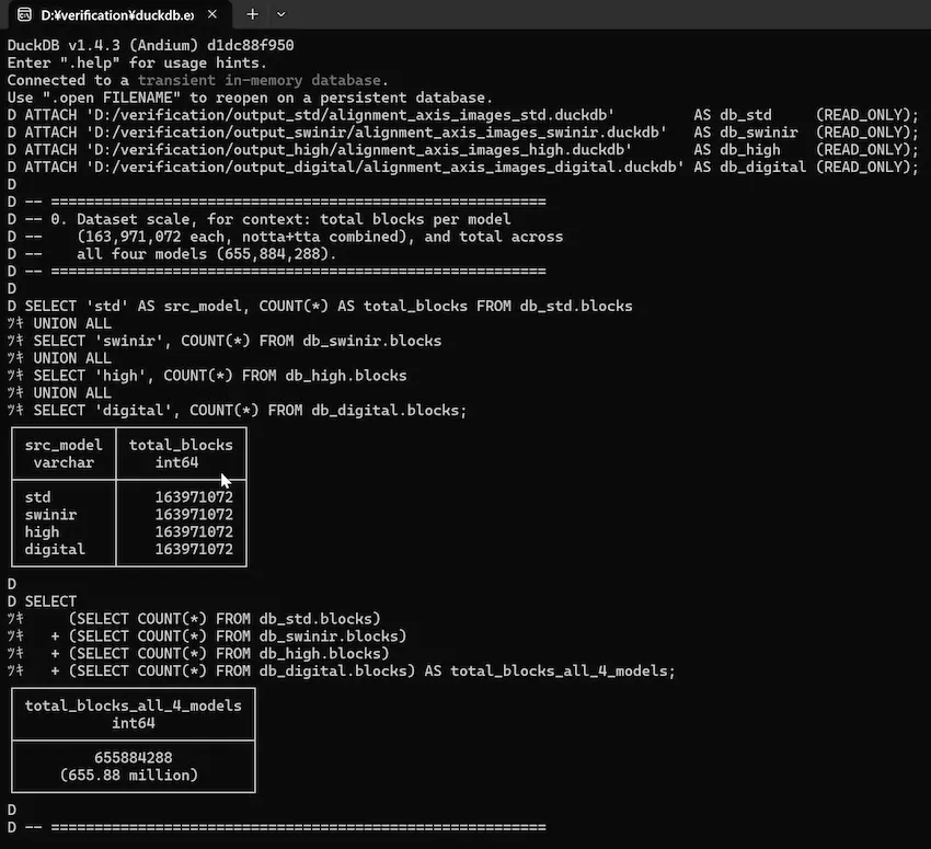
A DuckDB CLI session with all four models' databases ATTACHed together, showing a per-model block count of 163,971,072 each and a combined total of 655,884,288 blocks. — A real DuckDB CLI session, all four models' databases ATTACHed together — 655.88 million blocks, queried live on an ordinary PC.

DuckDB is often described as "SQLite for analytics." Where SQLite is optimized for transactional, row-by-row reads and writes on modest amounts of data, DuckDB uses column-oriented storage and an execution model built specifically for scanning and aggregating large volumes of data — designed from the ground up for analytical workloads. And like SQLite, it's an embedded database with no server process to run, so it works entirely on a single PC. Learning about that design philosophy, and recognizing how well it matched what we needed, is what made us decide to try it.

DuckDB's development is overseen by the DuckDB Foundation (Stichting DuckDB Foundation), an independent non-profit based in the Netherlands. Its directors are Hannes Mühleisen, Mark Raasveldt, and Peter Boncz, with companies including AWS, MotherDuck, and Posit sponsoring its development.

A less common pairing: DuckDB + a live 3D viewer

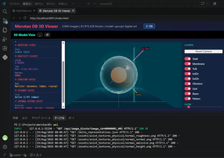
DuckDB-powered interactive visualization in the browser isn't unusual by itself — frameworks like Mosaic and MotherDuck's own case studies show it driving 2D charts over tens of millions of rows, typically via DuckDB-Wasm running inside the browser itself. What we haven't found precedent for is the more specific combination we use for our 3D block viewer: everything runs on a single local PC, no cloud involved — a local FastAPI web server queries DuckDB directly (DuckDB isn't compiled into the browser here), and Three.js renders the results as a 3D visualization, mapping roughly 16–20 dimensions of failure-related information onto independent visual channels of an egg-shaped model, without any dimensionality reduction. As far as we've found, that particular combination was an unusual way to use DuckDB as of August 2026.

VS Code showing the Merutan DB 3D Viewer running in a browser panel, with the egg-shaped 3D model (Shell/Membrane/Yolk) rendered on the right and a terminal below showing live FastAPI server request logs. — The viewer actually running: VS Code, the live 3D render, and the local FastAPI server's request log, all in one shot.

Why SQL

Another deciding factor was being able to run the entire analysis in plain SQL, without going through the custom Python libraries we'd relied on before. Analysis code written in a general-purpose language tends to invite suspicion the more complex it gets — is something being altered behind the scenes? A SQL statement is different: what it computes is right there in the query itself, and a third party can reproduce the same result simply by running the same query. That clarity, and that ease of verification, mattered to us.

Video evidence practices

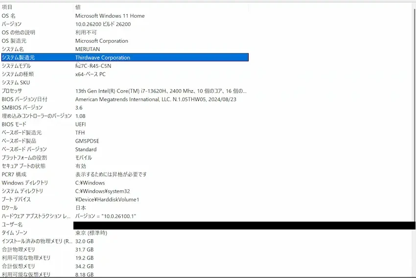
In practice, our technical report series publishes both the SQL statements themselves and a screen-recorded video of them running. But a video alone still leaves room for doubt — is this really running on a local PC? Partway through the series, we started opening each recording by showing the PC's system information (OS, specs) before recording the SQL running live.

Windows System Information panel showing OS version, CPU model, BIOS date, and memory, as shown at the start of one of our screen-recorded verification videos. — The system-info screen we open each recording with, proving it's a real local PC, not a fabricated result. (Username redacted for this page; the original video shows it unredacted.)

The no-join verification pipeline

Our original analysis setup joined a table of SSIM results with a separately-generated table of comp_* features, matched by coordinate. That join process turned out to be a recurring source of data-integrity bugs — rows that silently stayed at zero when they shouldn't have, or values from the wrong block ending up attached to the wrong row. Some of these bugs weren't even catchable with simple checks.

What made this tricky was that, using the same pipeline, some databases came out correct and others didn't. At a scale of hundreds of millions of rows, that kind of partial inconsistency isn't something you can spot by eye — it can sit there undetected indefinitely. That's why, rather than patching individual bugs as they turned up, we removed the join mechanism itself, switching to a design where this class of problem structurally can't occur.

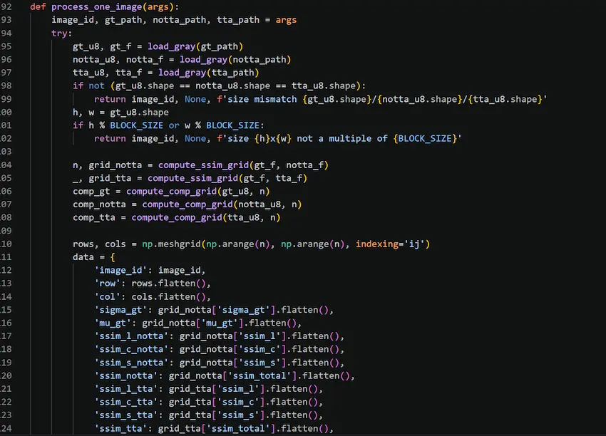
Our verification databases compute comp_* features and SSIM values directly from each reconstructed image in a single pass, without relying on joins across multiple tables. This structurally avoids a class of data-integrity bug (mismatched rows from JOINs) that we found repeatedly in an earlier, join-based database design. First established in DOI 1.12; see that report for full detail.

The exact code behind this design (build_notta_tta_comp_db.py and heatmap_tool.py) is released in full as DOI 1.19.1, together with a demonstration video. See Building the verification databases for how to run it on your own data, or the beginner-friendly code walkthrough for a section-by-section explanation of how it works.

Python source code for process_one_image(), loading the GT, noTTA, and TTA images and computing SSIM and comp_* feature grids directly from them in one pass, with no database join anywhere in the function. — The actual code: SSIM and comp_* values, computed directly from the loaded images — no join, no separate lookup step.

The comp_* feature framework

Eight reconstruction-side features (sharpness, edges, artifacts, contrast, texture, entropy, noise) that diagnose block-level structural and textural quality — the dimensions SSIM alone cannot fully capture. Full definitions and implementation are documented in DOI 1.8.

One of these eight turned out to have a use nobody had planned for: comp_contrast, divided by 255, is an exact, error-free measurement of a model's own reconstructed contrast — used in DOI 1.20.1 to flag SSIM Structural Masking risk without ground truth at all. See the plain-language explainer for that result and a companion GT-free tool for SSIM's other named blind spot.

We publish the full mathematical definitions and implementation code for all 8 comp_* features. Making exactly what's being computed and how transparent isn't just easier for readers to follow — it's also open science in practice.

This 8-feature set is not meant to be the final word. The comp_* framework and the DB-building pipeline (released in Technical Report v1.19.1) are both designed so that a developer can add their own diagnostic feature to the same condition set and build an evaluation tool tailored to their own use case. We'd like to see more skilled developers get involved in this kind of work — treating image-quality-metric reliability as part of the broader AI security conversation, not a separate concern.